Study of vibration

Fourier transform
So far we have only seen vibrations in the time domain, which are signals captured directly from the machine. As we said before, these signals contain all information about the behavior of each machine component. However, there is a problem when making fault diagnosis: these signals are loaded with a lot of information in a very complex form, including the characteristic signals of each individual machine component, so it is practically impossible to distinguish with the naked eye its characteristic behavior.
There are other ways to perform a study of vibrations, among which is to analyze the signals in the frequency domain. For this, the amplitude vs frequency plot is used, which is known as the spectrum. This is the best tool currently available for machinery analysis. It was precisely the French mathematician Jean Baptiste Fourier (1768 - 1830) who found a way to represent a complex signal in the time domain by means of series of sinusoidal curves with specific amplitude and frequency values.
So what a spectrum analyzer, working with the fast Fourier transform, is doing is to capture a signal from a machine, calculate all the series of sinusoidal signals contained in the complex signal and finally display them individually in a spectrum plot.
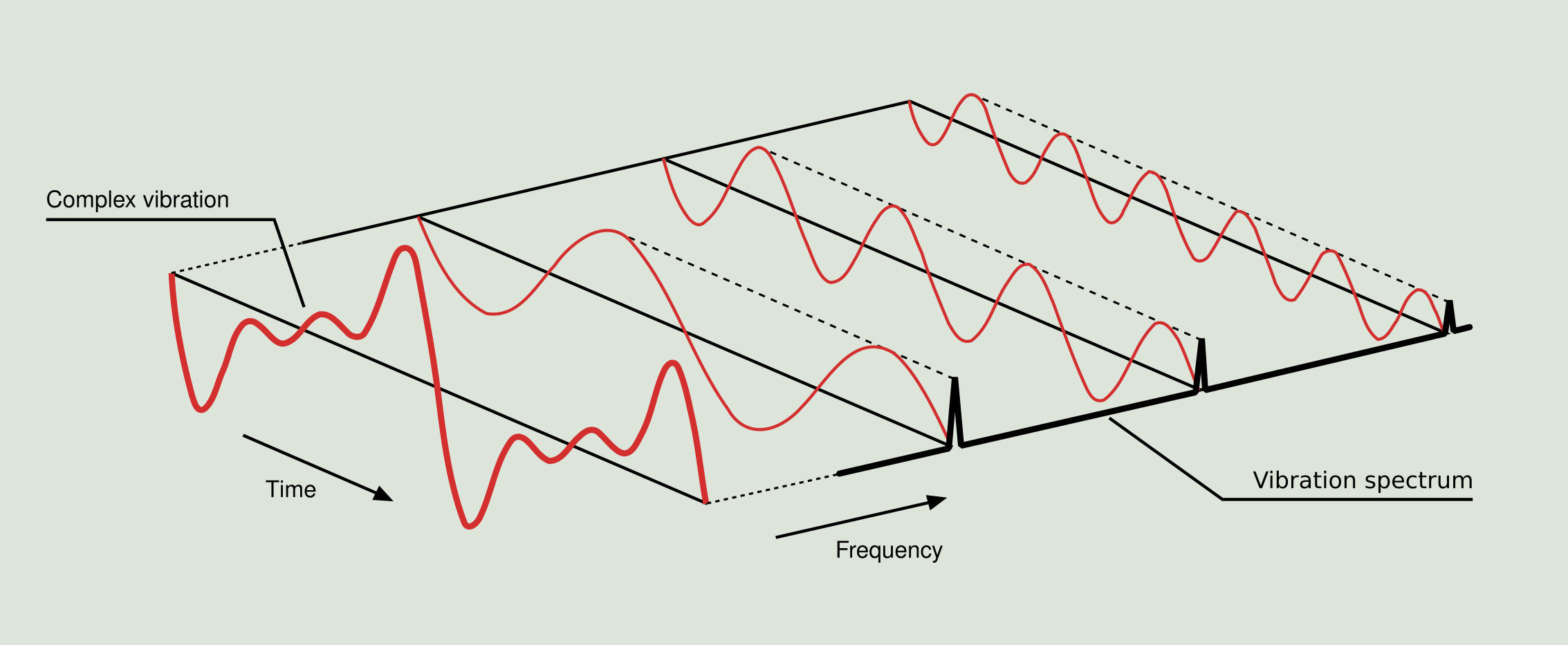
Figure 2.9 clearly shows a three-dimensional representation of the complex vibration signal acquired at a certain point in a machine. For this signal all the time domain sinusoidal signals that compose it are calculated, and finally each one of them is shown in the frequency domain.
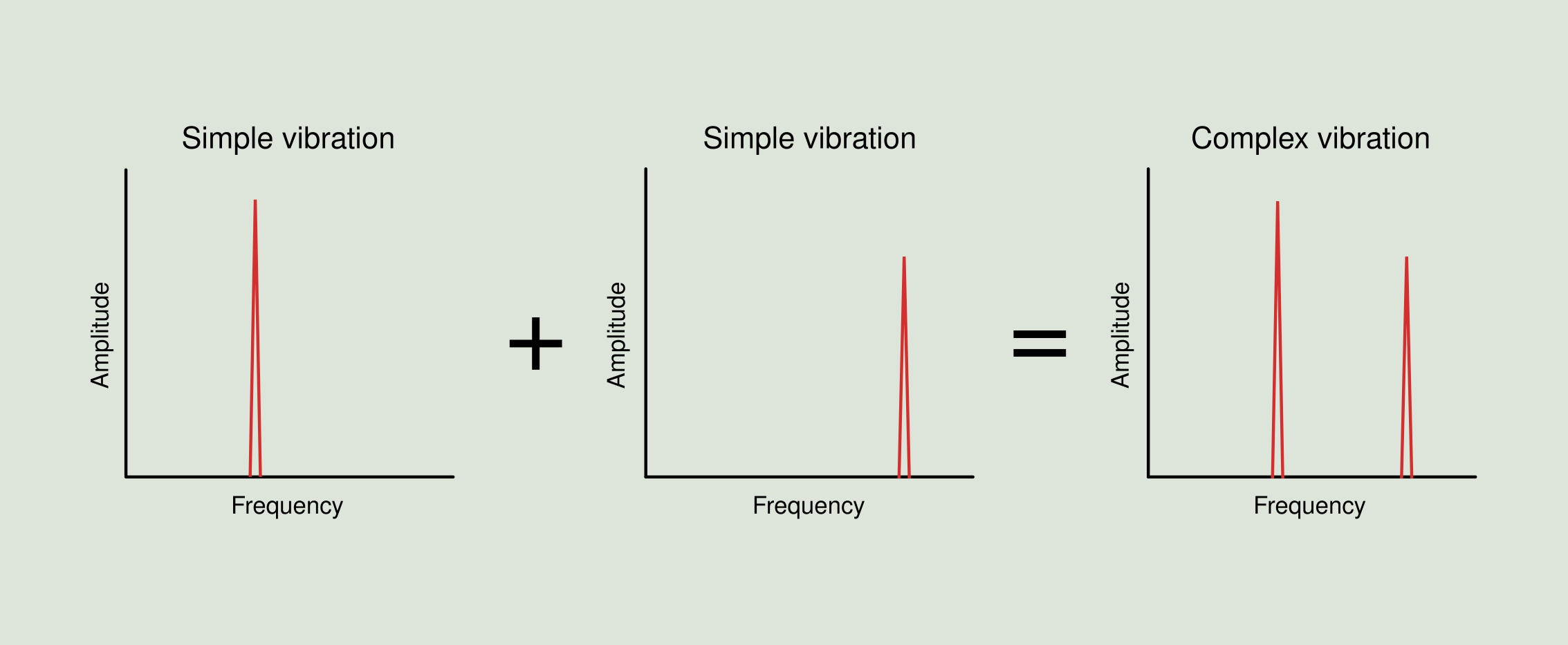
Therefore, by using the Fourier transform, we can retrieve the sum of simple vibrations from Figure 2.5 and represent exactly the same operation in the frequency domain as shown in Figure 2.10, with the particularity that in this case it is straightforward to obtain from the resulting spectrum the frequencies and amplitudes for the two original components.
As already mentioned, the time domain plot is called the waveform, and the frequency domain plot is called the spectrum. Spectrum analysis is equivalent to transforming the time domain signal information into the frequency domain. A clear example of equivalence in both domains is a time table, where we can say that a train leaves at 6:00, 6:20, 6:40, 7:00, 7:20, or we can say that a train leaves every 20 minutes beginning at 6:00 (this last figure representing the phase). The first option would be the time domain representation and the second one the frequency domain representation. The frequency domain representation brings, in comparison with the time domain, a reduction in the amount of data. The information is exactly the same in both domains, but in the frequency domain is displayed in a more compact and practical way.
Displacement, velocity and acceleration
So far, we have considered only displacement as a measurement of an object vibration amplitude. The displacement is simply the distance to the object from a reference position or equilibrium point. Apart from a variable displacement, a vibrating object has a variable velocity and a variable acceleration. Velocity is defined as the rate of change in displacement and is usually measured in in/s (inches per second) or mm/s. Acceleration is defined as the rate of change in velocity and is measured in g (the average acceleration due to gravity at the earth's surface) or mm/s². As we have seen, the displacement of a body that is subjected to a simple harmonic motion is a sinusoidal wave. Also both the velocity and acceleration curves of this motion are sinusoidal waves.
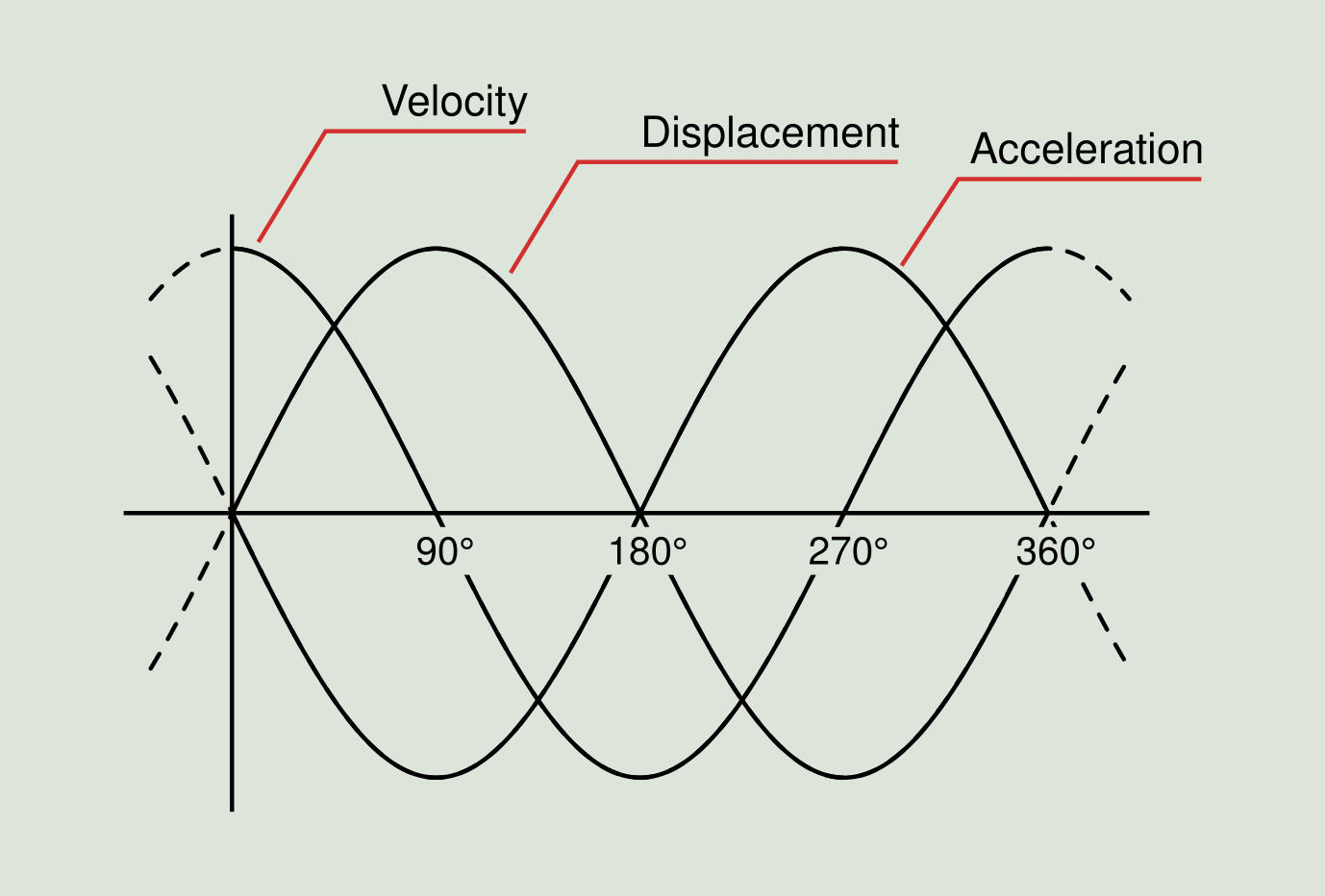
When the displacement reaches its maximum value, then the velocity is zero, because that is the location where the movement direction is reversed. When the displacement is zero (at the rest position), the velocity will reach its maximum value. This means that the velocity wave phase is shifted to the left by 90 degrees, compared to the displacement waveform. In other words, velocity is advanced 90 degrees with respect to displacement. Acceleration is the rate of change of velocity. When the velocity reaches its maximum, then the acceleration is zero because the velocity does not change at that moment. When the velocity is zero, then the acceleration is at its maximum since at that moment is when velocity changes the fastest. The sinusoidal curve of the acceleration as a function of time can thus be considered as to be shifted in phase to the left relative to the velocity curve and therefore acceleration has a 90 degree advance with respect to velocity and 180 degrees with respect to displacement.
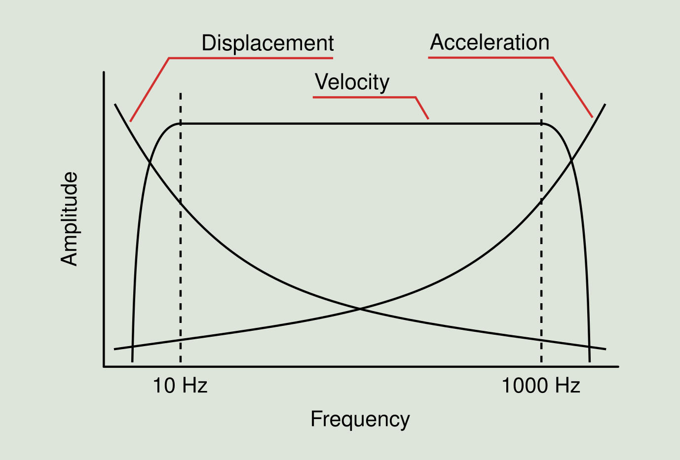
The amplitude units selected to express each measurement have a great influence on the clarity with which the vibration phenomena is manifested. Thus, as can be seen in Figure 2.12, the displacement shows its greatest amplitudes at low frequencies (typically below 10 Hz), the velocity does it at an intermediate range of frequencies (between 10 and 1,000 Hz), and acceleration is best expressed at high frequencies (above 1,000 Hz).
To illustrate these relationships, let us consider how easy it is to move one hand the distance of a palm at a cycle per second or 1 Hz. It would probably be possible to achieve a similar movement of the hand at 5 or 6 Hz. But think about the velocity at which you should move your hand to achieve the same displacement of a palm at 100 Hz or 1,000 Hz. This is why you never see high frequency levels combined with high displacement values. The enormous forces that would be needed simply do not occur in practice.
Figure 2.13 contains several plots showing an example of the behavior of the different amplitude units throughout the frequency range. The three spectra provide the same information, but their emphasis has changed. The displacement curve is more difficult to read at higher frequencies. The speed curve is the most uniform across the frequency range.
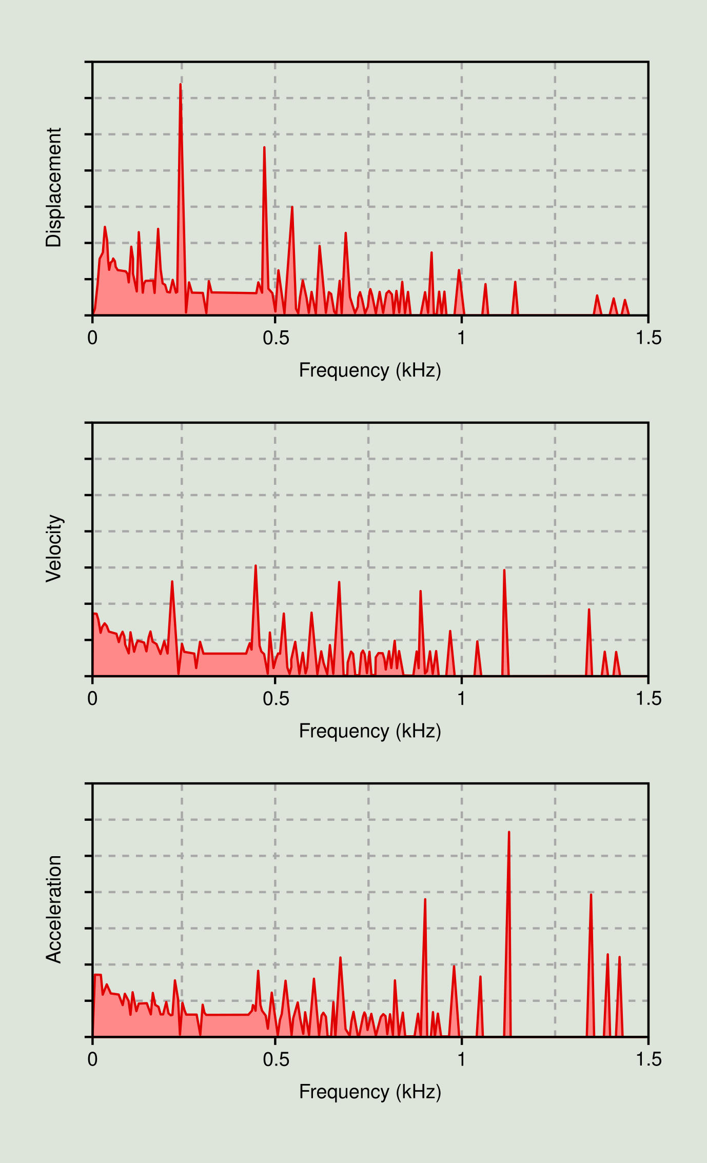
This is the typical behavior for most rotary machines, but in some cases the displacement and acceleration curves will be the most uniform. It is a good idea to select the units in such a way that you get the flattest curve. That provides the most visual information to the observer. The vibration parameter that is most commonly used in machinery diagnosis is velocity.
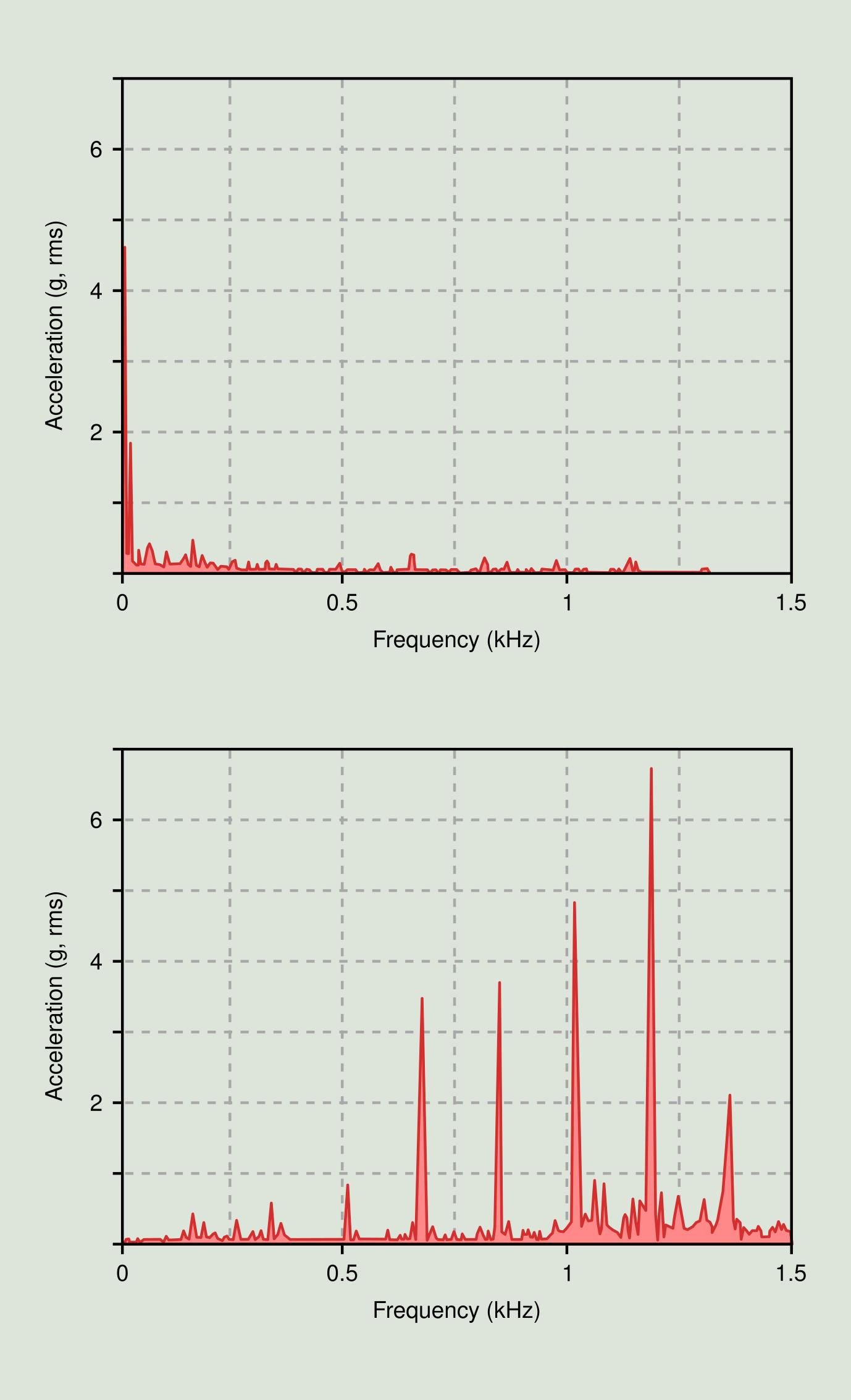
Finally, we illustrate what has been said so far with the practical case of the following figure where the same spectrum is shown in unit of displacement and acceleration. Both plots correspond to a deteriorated bearing. In the velocity spectrum the problem is not observed, whereas in the acceleration spectrum it is clearly observed.
Spectral analysis
When measuring the vibration of a machine, a lot of valuable information is produced that needs to be analyzed. The success of this analysis depends on the correct interpretation of the measured spectra with respect to the machine operating conditions. Typical steps in vibration analysis are:
-
Identification of vibration spectrum peaks: the first step is to identify the first order peak (1X), corresponding to the rotation speed of the machine shaft. In machines with multiple shafts, each shaft will have its characteristic rotational 1X frequency. In many cases, the peaks at 1X of the shaft are accompanied by a series of harmonics or integers multiples of 1X. There are harmonics of special interest, for example, in a six-vane pump, there will usually be a strong spectral peak at 6X.
-
Machine diagnosis: determination of the severity of the machine diagnosed issues based on the amplitudes and the relationship between the vibration peaks.
-
Appropriate recommendations for repairs, based on the severity of the machine issues.
Let us consider the example of the mechanical system of Figure 2.15.
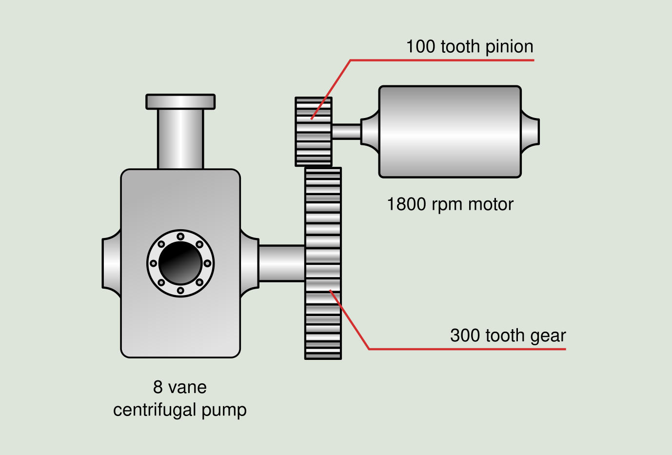
From the machine data provided it is possible to calculate the main frequencies of interest:
`sf "Motor turning frequency"`
` = sf "1,800 rpm" = sf "30 Hz"`
`sf "Pump turning frequency"`
` = sf "100 teeth" / sf "300 teeth" xx sf "1,800 rpm"`
` = sf "600 rpm" = sf "10 Hz"`
`sf "Gear mesh frequency"`
` = sf "100 teeth" xx sf "1.800 rpm"`
` = sf "300 teeth" xx sf "600 rpm"`
` = sf " 1.800.000 rpm"`
` = sf " 3.000 Hz"`
`sf "Vane pass frequency"`
` = sf "8 vanes" xx sf "600 rpm"`
` = sf "4.800 rpm" = sf "80 Hz"`
In this machine we have two axles (motor and pump). In the case of the motor, the value 1X is 30 Hz, in addition we will probably find a frequency peak in the spectrum in the harmonic 100X, which corresponds to the frequency of gearwheel between pinion and crown. For the pump, the value 1X is 10 Hz, and its main harmonic of interest is 8X, which corresponds to the pitch frequency. Obviously, other frequencies, such as side bands on the frequency of the gear, bearing frequencies, and harmonics of the calculated frequencies may appear.
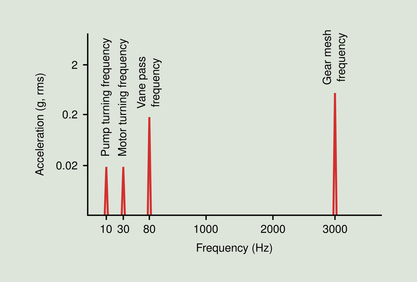
In the spectrum plot of Figure 2.16 is shown the vibration signature of our mechanical system example.
Once we have identified the frequencies of interest, the next question is whether the amplitude values are acceptable or unacceptable. An acceptable vibration value is one that does not cause a reduction in the useful life of the machine or cause damage to nearby equipment. Some machines are designed to tolerate extremely high vibration levels (eg mils) and other equipment are very sensitive even at the slightest level of vibration (eg optical systems). There are four ways to determine which vibration level is appropriate for a given machine. The best way is to keep a record of data over time for the critical machine points, and from this data establish benchmarks for acceptable levels. If there are several identical machines in the plant a second method can be used. If three machines show similar spectrum amplitudes and the fourth machine shows much higher levels working under the same conditions, it is easy to conclude which machine is having problems. Another method is to collect vibration data and send it to the manufacturer for evaluation. It must be taken into account that the vibration varies according to the working conditions and the installation of the machine. The fourth method is to choose a standard based on the experience of others and if necessary to adapt it based on your experience.